Distance Vector Routing Algorithms & The Count To Infinity Problem

Context

Routing is a fundamental building block of modern day computer networking. There are billions of devices and servers around the world. So when two devices wish to communicate with each other, how does data travel between them? The data is first broken into chunks, called packets, and each packet is transported one by one. We cannot have a direct communication link between the two devices. Think about it. With billions of existing devices, and many more being added daily, it would be nearly impossible and super inefficient to have direct links between each pair of devices.

So how do two devices transfer data between each other? The answer is through switches. Switches are of two types: packet switches and routers. These form the core of the internet, with the host devices and servers running on the edge. Routers, like the term suggests, route incoming data packets to the next router, and eventually to the destination. Each data packet has some metadata using which the router decides which output port it should be forwarded to. But, how does the router come up with the metadata-to-output port mapping? Before we answer this question, allow me to quickly introduce you to the internet's layered architecture.

Modern-day internet communication works in a layered manner. According to the TCP/IP model, there are 5 main layers: Application layer, Transport layer, Network layer, Link layer, and Physical layer. For communication to happen, there has to be a sender and a receiver. On the sender side, data flows down the layers. Each layer adds its own headers or metadata to the packet before passing it to the layer below. The physical layer is responsible for actually transferring the data to the receiver's physical layer through a transmission medium. On the receiver end, data flows upwards. Each layer reads its metadata, and passes the packet to the appropriate location in the layer above.

Routers are part of the Network layer. The two primary functions this layer serves are forwarding and routing. Forwarding is a local operation that happens at each router. This ties back to our earlier example about a router receiving a data packet, reading the metadata, and 'forwarding' it to the correct output port. Routing, on the other hand, is a global operation. It is more about deciding what is the most optimal path between two devices. This is how a router knows the mapping between a packet's metadata and the correct output port. The resulting mapping that a routing algorithm creates is stored in a router's forwarding table. The next time it receives a new data packet, it refers to the forwarding table and forwards the packet to the correct output port.

Routing Algorithms

There are ways in which routing can be done: classical destination based routing, and SDN (Software Defined Networking) based routing. Destination based routing, as the name suggests, maps a packet's destination IP address and destination port number to an output port. There are two common types of destination-based routing algorithms - Link State Algorithm and Distance Vector Algorithm. SDN based routing on the other hand uses other metadata like the source IP address, source port number, transport protocol (TCP/UDP), etc. for mapping. In other words, destination-based routing is a specialized version of SDN-based routing.

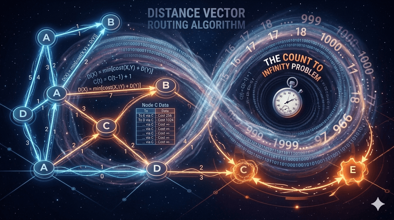
In this blog, we'll concentrate on destination-based routing, specifically the Distance Vector algorithm. We'll first see how the algorithm works, and then look at the Count To Infinity problem, something that I found quite fascinating when I first learnt about it.

How Does The Distance Vector Algorithm Work?

The distance vector algorithm is based on the Bellman-Ford equation:

To simplify, the source X looks at all its neighbors, compares their distances to the destination, and chooses the neighbor for which the distance from the source to the neighbor plus the distance from the neighbor to the destination is the least.

Each node (router) in the network maintains a distance vector, which is a list of its distances to other nodes in the network. From time to time, each node sends its own distance vector to its neighbors. When a node X receives new distance vector estimates from its neighbor Y, it updates its own distance vector using the Bellman-Ford equation. Basically, X checks if it can reach other nodes via Y with a lesser total cost, and if so, updates its own distance vector. Under natural conditions, the distance vector estimates converge to the actual least costs.

The following series of images demonstrate how the distance vector algorithm works over a very simple example.

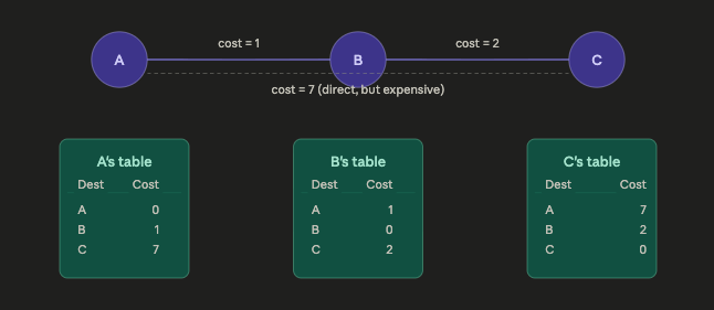
Step 0: Initialization of a three node network. Every node only knows about its neighbors.

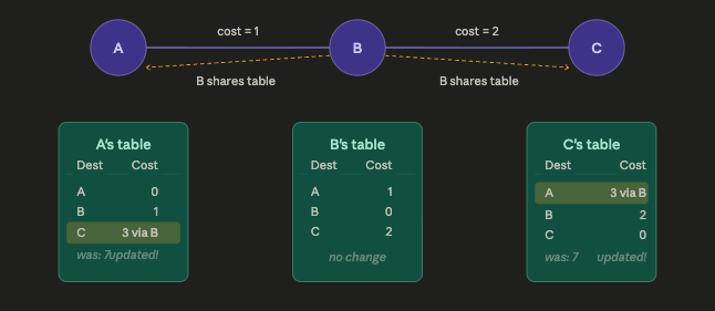
Step 1: Node B advertises its distance vector to its neighbors. Nodes A & C learn about paths to each other via B. They compare it with direct paths, and pick the minimum cost paths.

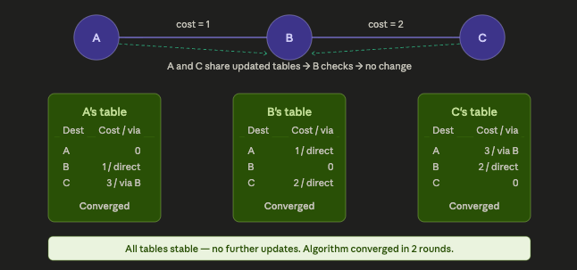
Step 2: Nodes A & C advertise their distance vectors to their neighbors. Nothing changes this time; the algorithm has converged.

For a more comprehensive example, I'd recommend this video by Prof. Jim Kurose.

The Count-To-Infinity Problem

In the above example, the algorithm only took two steps to converge to the optimal distance vector estimates. Even in other complicated examples, the algorithm converges pretty quickly because each node advertises its distance vectors to its neighbors; so information about a low-cost link spreads quickly. This phenomenon is called "good news travels fast."

But, what happens if a link cost suddenly increases? Does this information also travel as quickly? Not quite. Let's look at an example:

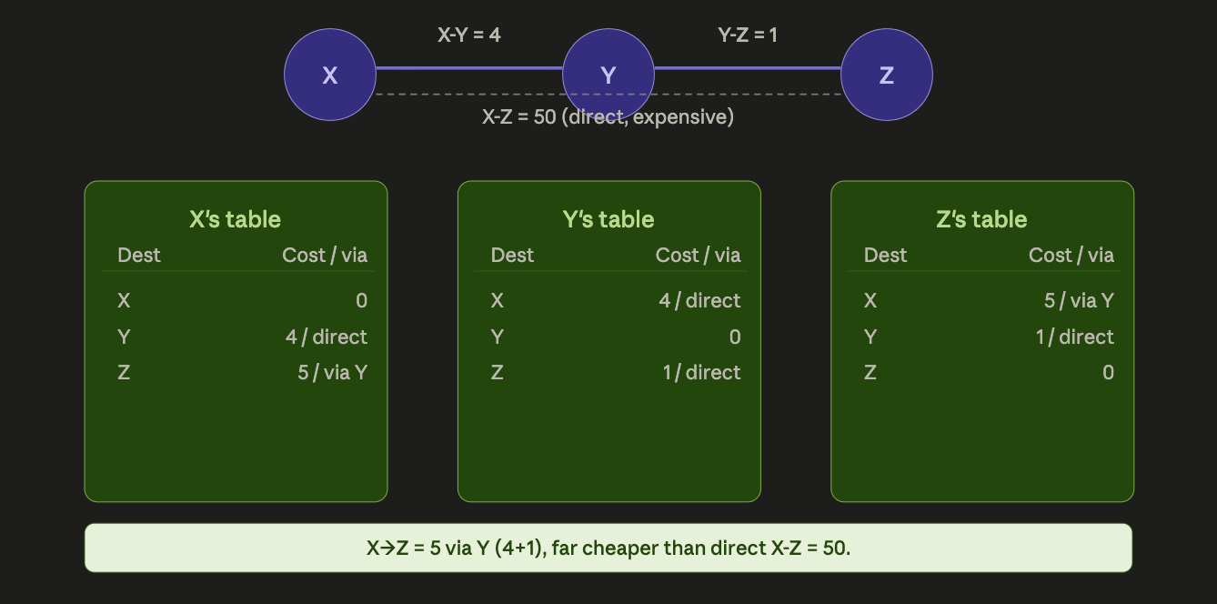
Step 0: Consider another 3 node network. Currently, all the routers have the optimal distance vectors.

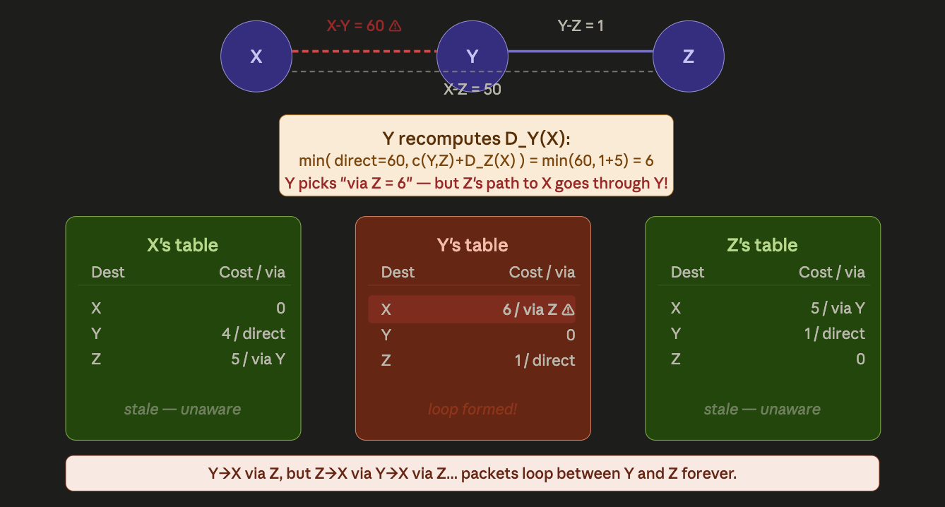
Step 1: Now the X-Y link cost increases to 60. Node Y now recomputes its distance to X. It compares its direct distance to X vs the distance via node Z and picks the minimum. But remember that Node Z's distance to X is via Y. So this creates a temporary loop. After Y recomputes its distance vector, it advertises it to its neighbors.

Step 2: Similarly, Z now recomputes its distance vector. It compares the direct cost to X vs the cost via node Y, and picks the minimum. Once again, Y's cost to X goes via Z creating a temporary loop. After Z recomputes its distance vector, it advertises it to its neighbors.

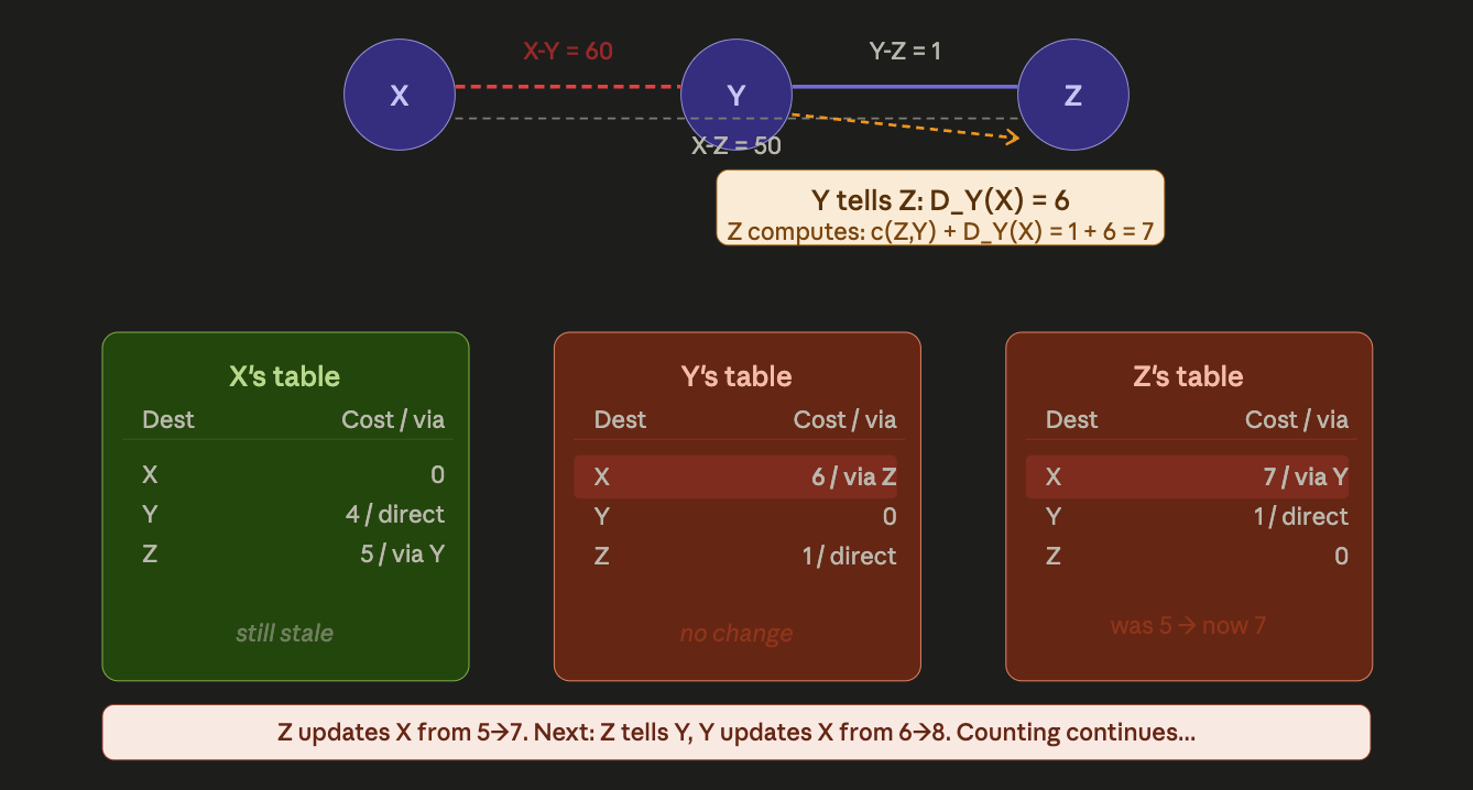
Step 3, 4, 5, and so on: Steps 1 & 2 repeat until the algorithm converges. Each step only increments the distances by 1, which is why it takes nearly forever for the algorithm to converge. At the end, we get the following distance vectors:

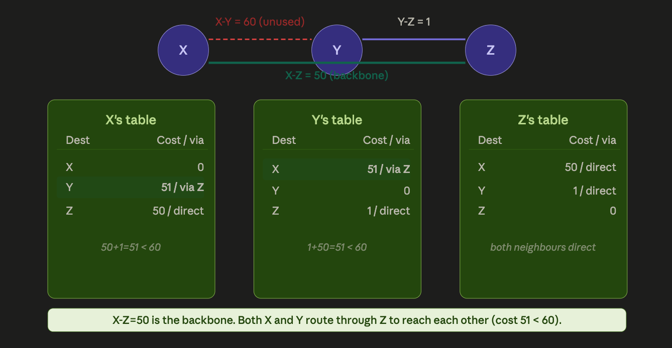
In this example, even though it takes a long time, the algorithm still converges. But imagine a scenario where the X-Y link breaks. It would be equivalent to setting its cost to infinity. In this case, the algorithm will never converge, which could be devastating.

How To Mitigate the Count to Infinity Problem?

There are three common practices used to prevent the count to infinity problem:

1. Split Horizon: Never advertise a route back to the neighbor you learned it from. In our example, Z learned about X via Y, so when Z advertises to Y it sets $D_Z(X) = \infty$. Y can no longer use Z as a fake shortcut and immediately accepts the true cost to X (direct link). This solution is simple and cheap, but only works for loops involving 2 nodes. It breaks down in larger loops (e.g. X→Y→Z→X).

2. Split Horizon with Poison Reverse: This is a stronger version of split horizon. Instead of simply omitting the route, Z actively advertises $D_Z(X) = \infty$ back to Y, i.e. "poisons" it. The result is the same, but the explicit poisoning makes convergence faster because Y immediately knows the route is dead rather than waiting for a timeout. This solution still doesn't solve loops of 3 or more nodes.

3. Maximum Hop Count (Count to Infinity Bound): Define a maximum cost and treat anything at or above it as infinity (i.e. unreachable). This doesn't prevent the counting, but it limits how long it goes on. Instead of counting forever, nodes converge after hitting the ceiling. The downside is that it caps the size of networks you can use the protocol in. Eg: RIP, a routing protocol can't support paths longer than 15 hops.

In practice, real protocols combine all of these solutions. Modern protocols like OSPF and BGP avoid the problem entirely by using link-state or path-vector algorithms instead of distance vectors, so nodes have full topology knowledge and can detect loops before they form.

Conclusion

The count to infinity problem is a great example of how a theoretically sound algorithm can run into very real practical challenges. The distance vector algorithm is elegant in its simplicity. But the locality of knowledge becomes its Achilles' heel when bad news strikes. A single link cost change can send routers into a prolonged disagreement, counting upward while real packets are silently dropped in the process. The mitigations chip away at the problem, but none fully solve it. This is ultimately why modern large-scale routing protocols like OSPF and BGP moved away from distance vectors entirely. Sometimes the cleanest fix is to rethink the foundation.

If you found this blog interesting, the broader world of routing algorithms is well worth exploring. I intend to cover more routing algorithms and other networking concepts in future blogs. Until then, may your packets always find their paths.